Design and Train a Graph Neural Model
This section showcases how a design and implement a graph-convolution based neural network for neuron classification. This will hopefully help the user to create their own models and carry out training experiments.
We will go through the whole process step by step while providing code samples that illustrate the concrete steps. To run any of the code samples the following import block needs to be included at the beginning of your python file:
import pathlib

import matplotlib.pyplot as plt
import torch
import torch.nn
import torch.optim
from morphoclass import data, layers, metrics, transforms, vis
from sklearn.metrics import accuracy_score
from torch.nn import functional as nnf
from torch_geometric.nn import ChebConv, GCNConv


plt.style.use("default")
Data
Any model design starts with the preparation of the data. Let us assume that a number of labeled neuron morphologies is available, and that these morphologies have been split into a training and a validation set. The corresponding filenames and labels have been saved in two separate CSV files:
data_dir = pathlib.Path("my_data")
train_csv = data_dir / "morphologies_training.csv"
val_csv = data_dir / "morphologies_validation.csv"
Note that both the training and validation sets need to be labeled, which is why the CSV files have to contain two columns – one with the file paths, and one with the labels, see the Data section for more details.
Next we need to decide how to pre-process the data, and which data features to use for training and evaluation. In this example we would like to carry out the following steps:
Load the apical trees
Simplify those trees to only the branching nodes
Extract first feature: the path distance from the soma to the nodes
Extract the second feature: the apical tree diameters at nodes.
As described in the Data section we need to define transforms that will transform the raw input morphologies to the features just described:
morphology_loader = transforms.Compose([
    transforms.ExtractTMDNeurites(neurite_type='apical'),
    transforms.BranchingOnlyNeurites(),
    transforms.ExtractEdgeIndex(),
])

feature_extractor = transforms.Compose([
    transforms.ExtractPathDistances(),
    transforms.ExtractDiameters(),
])
Note the transforms.ExtractEdgeIndex() transform, that loads the adjacency matrix
that represents the connectivity of the apical tree. This is almost always necessary. The
reason why we split the transform pipeline into two steps will become clear shortly.
First let’s load the training dataset:
ds_train = data.MorphologyDataset.from_csv(
    train_csv,
    pre_transform=morphology_loader,
    transform=transforms.Compose([
        transforms.MakeCopy(keep_fields=["edge_index", "tmd_neurites", "x", "y", "y_str"]),
        feature_extractor,
    ]),
)
An important step in the feature extraction is the feature normalization. Usually neural networks don’t cope well with very big and very small numbers, which is why it is best to have the values of the features distributed around 1. For example’s sake let us create and fit two different scalers for each of the two features:
scaler_path_distances = transforms.FeatureRobustScaler(feature_indices=[0], with_centering=False)
scaler_diameters = transforms.FeatureMinMaxScaler(feature_indices=[1])

scaler_path_distances.fit(ds_train)
scaler_diameters.fit(ds_train)
Now these scalers need to be integrated into the transform pipeline. In the Data section
we showed that this can be done by replacing the transform attribute of the dataset
instance. Here we show a different method: the datasets can be reloaded from disk, but this
time with the transforms containing the fitted scalers:
total_transform = transforms.Compose([
    morphology_loader,
    feature_extractor,
    scaler_path_distances,
    scaler_diameters,
])

ds_train = data.MorphologyDataset.from_csv(
    train_csv,
    pre_transform=total_transform,
)

ds_val = data.MorphologyDataset.from_csv(
    val_csv,
    pre_transform=total_transform,
)
At this point it is useful to verify that the feature extraction was successful, and that the node feature values are in the expected range:
print(ds_val[0].x[:10])
This prints the values of both features for the first ten nodes of the first sample in the validation dataset and should give something similar to this:
tensor([[0.0000, 0.5136],
        [0.0115, 0.3226],
        [0.0198, 0.1009],
        [0.0358, 0.0604],
        [0.1336, 0.0306],
        [0.0484, 0.0405],
        [0.0984, 0.0199],
        [0.0522, 0.0306],
        [0.0567, 0.0199],
        [0.0655, 0.0199]])
The Net
The next step is to design a neural network that can operate on our data and produce a prediction for the morphology type. Unfortunately there is no simple design recipe and it is the experience of the researcher and the results of experimentation with different network architectures that determine the final layout of the network. The final network design could look something like this:
class MyNet(torch.nn.Module):

    def __init__(self, n_features, n_classes):
        super().__init__()
        self.conv_1 = ChebConv(n_features, 128, K=5)
        self.conv_2 = GCNConv(128, 256)
        self.conv_3 = GCNConv(256, 512)
        self.pool = layers.AttentionGlobalPool(512)
        self.fc = torch.nn.Linear(512, n_classes)

    def forward(self, data):
        x = data.x
        edge_index = data.edge_index

        x = self.conv_1(x, edge_index)
        x = nnf.relu(x)
        x = self.conv_2(x, edge_index)
        x = nnf.relu(x)
        x = self.conv_3(x, edge_index)
        x = nnf.relu(x)
        x = self.pool(x, data.batch)
        x = self.fc(x)
        x = nnf.log_softmax(x, dim=1)

        return x
Let us break down the important steps. A typical neural net will inherit from the
torch.nn.Module class, and overload the forward method that defines the forward
pass through the network. This method should have one parameter – the input data. More
precisely these will be batches of samples that we loaded using the MorphologyDataset
class above. Note that this dataset class takes care of correctly creating the batches.
In the constructor we define the different layers that the data will flow through in the forward pass. We use ChebConv and GCNConv graph convolution layers for node feature extraction. These will be followed by an attention global pooling layer that will summarize features of all nodes in an apical tree into one feature vector. Finally, a fully connected layer will transform this feature vector into a probability distribution over the morphology type classes.
One can see in the forward pass that the various steps are interlaced with the application of the ReLU non-linearity and that the final activations are passed through a softmax layer to produce logarithmic probabilities.
To design your own nets it is useful to use third-party libraries that implement the network layers. A great resource is the PyTorch-Geometric that we also use in this example.
The Training Loop
The next step is to set up a training loop that will instantiate and train our custom net.
First create an instance of the network and an optimizer:
device = torch.device("cuda" if torch.cuda.is_available() else "cpu")
n_classes = len(ds_train.class_dict)

net = MyNet(n_features=2, n_classes=n_classes)
net = net.to(device)

optimizer = torch.optim.SGD(net.parameters(), lr=1e-2)
Here we choose the SGD for the optimizer, but as with the design of the net there are many possible choices here as well and often the best choice can only be determined by experimentation.
Finally let us spell out the training loop. The following structure is very typical:
results = {
    "train_acc": [],
    "train_loss": [],
    "val_acc": [],
    "val_loss": [],
}

train_loader = data.MorphologyDataLoader(ds_train, batch_size=16, shuffle=True)

for epoch in range(1500):
    # Train
    net.train()
    for batch in train_loader:
        batch = batch.to(device)
        optimizer.zero_grad()
        out = net(batch)
        loss = nnf.nll_loss(out, batch.y)
        loss.backward()
        optimizer.step()

    # Evaluate
    net.eval()
    train_acc, train_loss = get_accuracy_and_loss(net, ds_train, device)
    val_acc, val_loss = get_accuracy_and_loss(net, ds_val, device)
    results["train_loss"].append(train_loss)
    results["train_acc"].append(train_acc)
    results["val_loss"].append(val_loss)
    results["val_acc"].append(val_acc)

    # Print info
    if (epoch + 1) % 10 == 0:
        print(
            f"[epoch {epoch + 1:3d}] "
            f"train_loss={train_loss:.2f} train_acc={train_acc:.2f} "
            f"val_loss={val_loss:.2f} val_acc={val_acc:.2f} "
        )
and the output that it produces might looks as follows:
[epoch  10] train_loss=1.35 train_acc=0.37 val_loss=1.35 val_acc=0.38
[epoch  20] train_loss=1.33 train_acc=0.37 val_loss=1.32 val_acc=0.38
[epoch  30] train_loss=1.32 train_acc=0.37 val_loss=1.30 val_acc=0.38
[epoch  40] train_loss=1.30 train_acc=0.37 val_loss=1.29 val_acc=0.38
[epoch  50] train_loss=1.29 train_acc=0.37 val_loss=1.26 val_acc=0.38
[epoch  60] train_loss=1.27 train_acc=0.37 val_loss=1.24 val_acc=0.38
[epoch  70] train_loss=1.25 train_acc=0.37 val_loss=1.21 val_acc=0.38
[epoch  80] train_loss=1.23 train_acc=0.37 val_loss=1.18 val_acc=0.38
[epoch  90] train_loss=1.20 train_acc=0.37 val_loss=1.15 val_acc=0.38
[epoch 100] train_loss=1.18 train_acc=0.40 val_loss=1.12 val_acc=0.38
[epoch 110] train_loss=1.16 train_acc=0.45 val_loss=1.09 val_acc=0.44
[epoch 120] train_loss=1.13 train_acc=0.49 val_loss=1.06 val_acc=0.56
...
[epoch 1470] train_loss=0.61 train_acc=0.76 val_loss=0.45 val_acc=0.81
[epoch 1480] train_loss=0.61 train_acc=0.75 val_loss=0.45 val_acc=0.75
[epoch 1490] train_loss=0.60 train_acc=0.77 val_loss=0.43 val_acc=0.81
[epoch 1500] train_loss=0.60 train_acc=0.77 val_loss=0.44 val_acc=0.81
In the first preparatory step we initialize a dictionary that will hold our training results, and a data loader that will generate batches of data from our training dataset.
After it we start the training loop with 1500 epochs that essentially consists of three different sub-steps: training, evaluation, and output on the screen. The code for these steps should be self-explanatory, and a similar structure of the training loop is widely used in the machine learning community.
There are a number of libraries that aim at removing the boiler-plate of the training loop
in PyTorch, the most notable at the moment are Ignite and PyTorch-Lighning. Also
morphoclass provides such abstractions, which we saw in for om the trainer classes in the
sections GNN, CNN, and PersLay.
You may have noted that above we used a helper function that computed the accuracies and losses on the training and validation sets. Here is its implementation:
def get_accuracy_and_loss(net, dataset, device):
    all_labels = []
    all_predictions = []
    all_losses = []
    net = net.to(device)
    loader = data.MorphologyDataLoader(dataset, batch_size=128)

    for batch in loader:
        batch = batch.to(device)
        log_probability = net(batch)
        prediction = log_probability.argmax(dim=1)
        label = batch.y
        loss = nnf.nll_loss(log_probability, label, reduction="none")

        all_labels.extend(label.tolist())
        all_predictions.extend(prediction.tolist())
        all_losses.extend(loss.tolist())

    accuracy = accuracy_score(all_labels, all_predictions)
    loss = sum(all_losses) / len(all_losses)

    return accuracy, loss
Similarly to the training loop at loops over batches of data using a data loader, computes the predictions by calling the forward pass of the net, and saves the results.
Visualizing Results
After the training loop has finished we can plot the results that we collected during the training loop:
fig, (ax_acc, ax_loss) = plt.subplots(1, 2, figsize=(10, 5))

ax_acc.set_title("Accuracies")
ax_acc.set_xlabel("Epoch")
ax_acc.set_ylabel("Accuracy")
ax_acc.set_ylim([0, 1])
ax_acc.plot(results["train_acc"], label="Train Accuracy")
ax_acc.plot(results["val_acc"], label="Validation Accuracy")
ax_acc.legend()

ax_loss.set_title("Losses")
ax_loss.set_xlabel("Epoch")
ax_loss.set_ylabel("Accuracy")
ax_loss.set_ylim([0, 2])
ax_loss.plot(results["train_loss"], label="Train Loss")
ax_loss.plot(results["val_loss"], label="Validation Loss")
ax_loss.legend()

fig.show()
A possible figure produced by this code might look as follows:
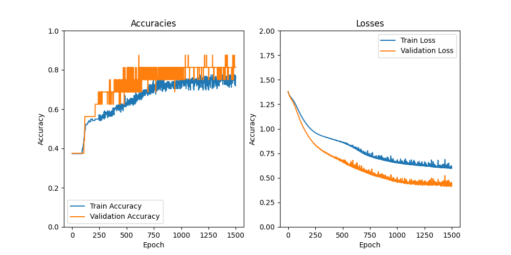
We can see that the model is learning something over time and that the loss is decreasing. The fact that the accuracy on the training set saturates below 80% is an indication that the choice of the network architecture and the training procedure might need to be improved.